This is Part 6 of the solution architecture series. Part 1 covered the five forces. Part 2 covered resilience. Part 3 covered delivery discipline. Part 4 walked through the scaling journey from 50 rps to 500,000. Part 5 covered the subsystems that hold. This is the reference card. Print it. Tape it near your desk.
In 2023, I watched an architect at a Fortune 500 healthcare company kill a $40 million initiative in a twenty-minute design review by writing one number on a whiteboard.
The team had proposed a real-time clinical-decision-support engine. It would score every incoming patient encounter against a deployed risk-prediction model, surface guideline-based recommendations, and return a ranked list of interventions to the clinician's screen in under 200 milliseconds. The diagrams were beautiful. There was a feature store, a model-serving tier, a Redis cache, a fallback layer. Someone had already named the service.
The architect asked one question. What's the traffic at peak?
Twelve thousand encounters per second across the hospital network's digital-front-door systems, the product manager said.
The architect turned to the whiteboard. He wrote:
12,000 rps × 86,400 seconds = ~1 billion inferences per day.
Then he wrote the model-serving cost he'd pulled from a back-of-envelope calculation the previous week — per inference, at scale, with retries. The number was big enough that the room went quiet. A month later, the project was quietly re-scoped to a nightly batch-precompute architecture that surfaced predictions from a lookup table at the point of care, and cost about 3% of the original plan.
He had not been smarter than anyone else in the room. He had carried two numbers in his head — the cost of a model inference, and the multiplier for turning QPS into daily volume — and that was enough to save forty million dollars.
This article is about the numbers every architect should carry. Not frameworks. Not diagrams. Numbers. The power of two that tells you a petabyte is about a million gigabytes. The latency of a disk seek versus an SSD fetch versus an L1 cache hit. The cost of a GPU-hour for training versus inference in 2026. The availability arithmetic that tells you what 99.99% actually costs over 99.9%.
The list that follows is the one I wish I'd had printed next to my monitor for the first ten years of my career. It is current as of April 2026. Cloud services change. Model pricing changes. The orders of magnitude do not.
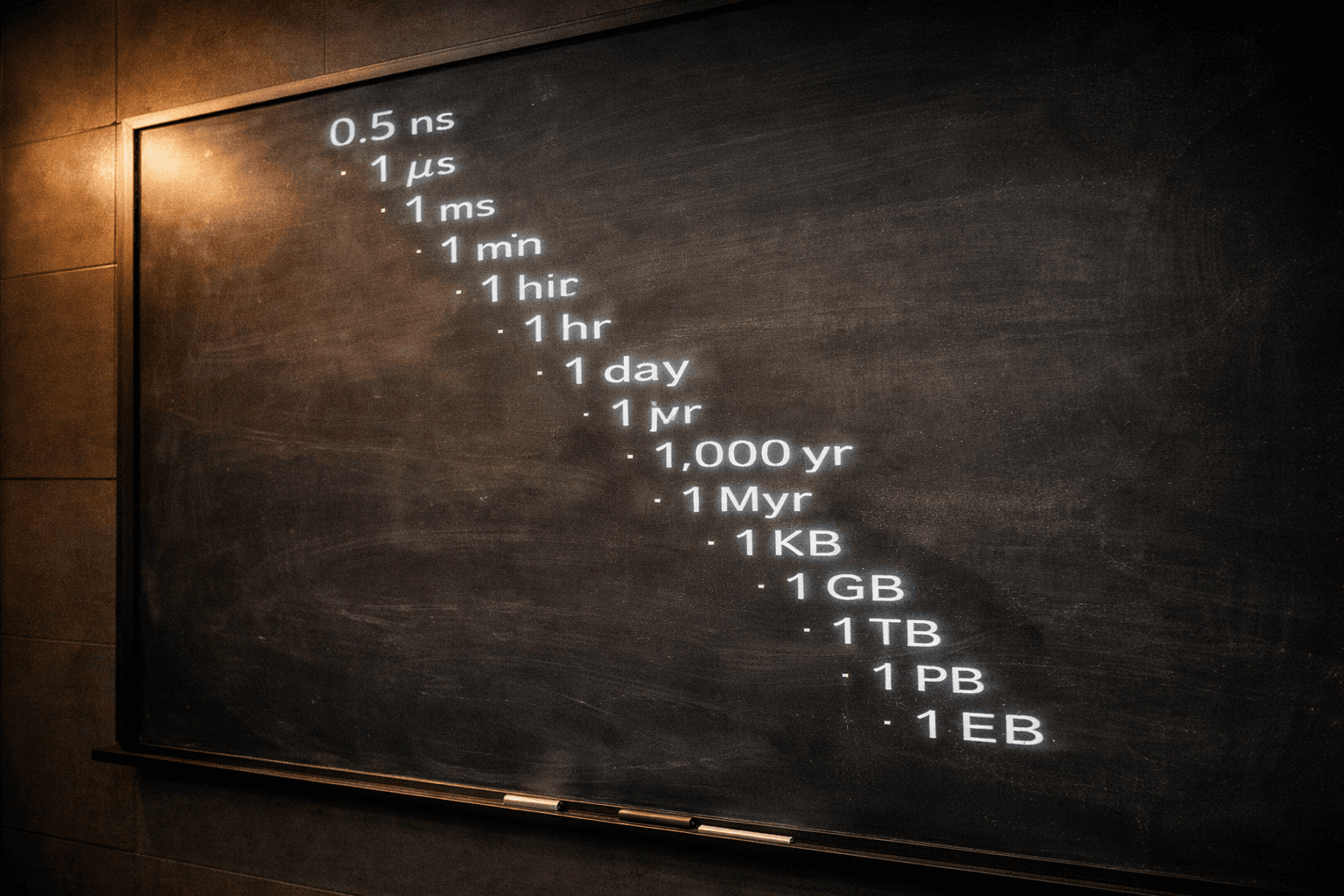
1. The Power of Two
Computers are binary. Sizes double. The faster you can translate between a power of two and the unit it refers to, the less time you lose squinting at Grafana axes or guessing whether a shard is going to overflow.
| Power | Value | Unit (approx) | Real-world sizing |
|---|---|---|---|
| 2¹⁰ | 1,024 | 1 KB | A single log line |
| 2²⁰ | ~1 million | 1 MB | A compiled microservice binary |
| 2³⁰ | ~1 billion | 1 GB | RAM in a laptop; a docker image layer |
| 2⁴⁰ | ~1 trillion | 1 TB | A full Postgres database for a medium SaaS |
| 2⁵⁰ | ~1 quadrillion | 1 PB | Data lake for a large enterprise |
| 2⁶⁰ | ~1 quintillion | 1 EB | Google Drive, approximately |
Two useful mental shortcuts:
- 1 million ≈ 2²⁰. So "10 million users × 1 KB profile" = 10 × 2²⁰ × 2¹⁰ = 10 GB.
- Halving your cache hit rate doubles your database load. Doubling your shards halves the per-shard hot-key pressure.
Where it shows up in real architecture decisions:
- Cache sizing. ElastiCache Redis r7g.4xlarge has 105 GB. If your working set is 2^36 bytes (~68 GB) and you're at 90% utilization, you are one hot-key eviction away from a cascade.
- TCP buffers. Default Linux send/receive buffers cap at ~4 MB. For high-bandwidth cross-AZ traffic you often need to raise these — the ceiling is a power-of-two choice.
- Database pages. Postgres default is 8 KB (2¹³). MySQL InnoDB is 16 KB. Every schema decision implicitly respects these boundaries.
2. Latency Numbers (2026 Cloud Edition)
Peter Norvig's "Latency Numbers Every Programmer Should Know" table is the most important reference card in distributed systems, and it hasn't been meaningfully updated for cloud since about 2012. Here is the current version, with cloud-specific additions that matter in 2026.
| Operation | Time | Order of magnitude |
|---|---|---|
| L1 cache reference | 0.5 ns | Nanoseconds |
| Branch mispredict | 3 ns | |
| L2 cache reference | 4 ns | |
| Mutex lock/unlock | 15 ns | |
| Main memory reference | 80 ns | |
| Compress 1 KB with Snappy | 2 μs | Microseconds |
| Read 1 KB from NVMe SSD | 5 μs | |
| Read 1 MB sequentially from DRAM | 40 μs | |
| Intra-AZ network round trip (AWS) | ~250 μs | |
| Read 1 MB sequentially from NVMe SSD | 500 μs | |
| Cross-AZ network round trip (AWS, same region) | ~1 ms | Milliseconds |
| ElastiCache Redis GET (in-AZ) | ~0.5 ms | |
| DynamoDB single-item read (p50) | 2–4 ms | |
| Aurora primary query (cached plan) | 1–3 ms | |
| S3 GET latency (p50, small object) | 15–30 ms | |
| Lambda warm invocation (p50) | 10–30 ms | |
| Lambda cold start (Java, 256MB) | 400–1500 ms | |
| Lambda SnapStart cold start | 100–300 ms | |
| Cross-region round trip (us-east-1 ↔ us-west-2) | ~60 ms | |
| Cross-continent round trip | 120–180 ms | |
| Claude Sonnet 4.6 streaming TTFT | 300–900 ms | |
| Claude Opus 4.7 streaming TTFT | 500–1500 ms | |
| GPT-5 streaming TTFT | 400–1200 ms | |
| Vector similarity search (~100M vectors, pgvector) | 50–200 ms | |
| Vector similarity search (Pinecone, same scale) | 20–80 ms | |
| GPU inference (Llama 70B on H200, batch 1) | 80–300 ms | |
| SQS send + receive (in-region) | 5–20 ms | |
| Kafka produce-to-consume (in-AZ) | 2–10 ms | |
| EventBridge custom event delivery | 50–100 ms | |
| SNS → SQS fan-out | 20–50 ms | |
| Istio sidecar proxy hop (per hop) | 2–5 ms | |
| EKS pod cold start (new container, image cached) | 3–10 sec | Seconds |
| EKS pod cold start (image pull, 500 MB) | 10–30 sec | |
| HPA scale-up (metrics lag + pod start) | 30–90 sec | |
| RDS Proxy connection acquisition | 1–5 ms | Milliseconds |
The distance between "things you can do inside one request" and "things that need to be async or precomputed" is somewhere around the 30 ms line. Anything below 30 ms is negotiable inside a user-facing request path. Anything above 30 ms is a design decision — caching, precomputation, streaming, or a promise to the user that they will wait.
Cloud-specific notes:
- AWS cross-AZ inside a region is ~1 ms. Design multi-AZ for availability, not for latency. If you are doing a synchronous cross-AZ read on every request, you are paying 1 ms per hop on traffic you did not need to pay for.
- AWS cross-region is ~60 ms coast-to-coast in the US, ~150 ms transcontinental. Multi-region active-active needs either eventual consistency or a CRDT-shaped data model. Multi-region active-passive needs a failover budget. Aurora DSQL (GA in 2025) changes this math — it provides strong consistency across regions but at a latency cost per write that you must budget for.
- Lambda cold starts are no longer a lost cause. SnapStart (for Java, .NET, and Python) cuts cold-start latency by an order of magnitude by snapshotting the initialized runtime. For Node.js, Provisioned Concurrency remains the answer when cold starts matter.
- Istio adds 2–5 ms per sidecar hop. A request that traverses three services in a mesh pays 6–15 ms in proxy overhead alone. If your p99 budget is 100 ms, that mesh tax is significant. Know your hop count.
- Kubernetes scaling is not instant. HPA reacts to metrics with a 15–30 second lag, then pods take 3–10 seconds to start (longer if image isn't cached). For bursty traffic, pre-scale or use KEDA with predictive scaling.
- Azure comparable numbers: Cosmos DB single-partition read ~5 ms p50 in same region. Azure Cache for Redis in-region RTT ~1 ms. Azure Functions Premium plan cold starts 200–800 ms. Azure Service Bus queue latency ~5–15 ms.
3. Availability Math
Nines are deceptive. They compress what's actually a logarithmic scale into something that reads like a linear one. Carry this table:
| Availability | Downtime / year | Downtime / month | What it means in practice |
|---|---|---|---|
| 99% | 3.65 days | 7.2 hours | Dev/staging, internal tools |
| 99.9% | 8.76 hours | 43.8 min | Most B2B SaaS |
| 99.95% | 4.38 hours | 21.9 min | Premium-tier SaaS SLA |
| 99.99% | 52.6 min | 4.4 min | Payment systems, trading floors |
| 99.999% | 5.26 min | 26 sec | Telecom, critical healthcare |
| 99.9999% | 31.5 sec | 2.6 sec | Rarely achievable for full applications |
The dependency multiplication trap. If your service depends on N components each at availability A, your theoretical ceiling is A^N. Five dependencies at 99.9% each gives you a theoretical ceiling of 99.5% (44 hours/year) — and that is before you add your own bugs.
The implication: every time someone says "let's add another service to the critical path," they are lowering your achievable nines. If you are chasing 99.99%, you have a maximum dependency budget measured in single digits, and every one of those dependencies has to operate at 99.995% or better. You do not get there by architecture drawings. You get there by ruthless pruning.
The real cost of a nine is not technical — it is political. Going from 99.9% to 99.99% usually means removing dependencies that someone built and is attached to. Going from 99.99% to 99.999% usually means rewriting the database layer or accepting regional failover as a first-class mechanism. Budget for the meetings, not the code.
4. The Estimation Framework: DAU → QPS → Storage → Cost
Most architecture mistakes trace to one missing chain in the conversion from human-scale numbers (users, documents, actions per day) to machine-scale numbers (queries per second, bytes, dollars per month). Here is the chain.
Step 1: DAU → QPS. If you have D daily active users and each user generates R requests per day, average QPS is:
Average QPS = (D × R) / 86,400
Peak QPS    = Average QPS × 2 to 3 (depending on traffic shape)
For a consumer app with a clear peak (evening in a timezone), use 3×. For a global B2B app with a flatter curve, use 2×.
Step 2: QPS → storage growth. If each request writes a record of size S:
Daily write volume = QPS × 86,400 × S × Write Ratio
Where Write Ratio is the fraction of requests that actually produce storage — typically 0.1 to 0.5 depending on the workload.
Step 3: Storage → cost. Pick the appropriate tier:
| AWS tier | Price per GB-month (2026) | Use case |
|---|---|---|
| S3 Standard | ~$0.023 | Active data |
| S3 Standard-IA | ~$0.0125 | Infrequently accessed |
| S3 Intelligent-Tiering | $0.023 + tier-out savings | Unpredictable access |
| S3 Glacier Instant Retrieval | ~$0.004 | Quarterly access |
| S3 Glacier Deep Archive | ~$0.00099 | Compliance, archive |
| EBS gp3 | ~$0.08 | Boot + transactional |
| Aurora Serverless v2 storage | ~$0.10 | Relational hot data |
Worked example: a URL shortener at scale.
Assumptions:
- 100 million DAU
- 10 URL-shortens per user per day + 100 URL-expands per user per day
- Each shortened URL stored at 500 bytes (URL + metadata + analytics pointer)
- Read:Write ratio = 10:1
- Peak factor 3×
Compute:
- Write QPS average = (100M × 10) / 86,400 = ~11,600 writes/sec
- Peak write QPS = ~35,000 writes/sec
- Daily new storage = 100M × 10 × 500 bytes = 500 GB/day
- Yearly new storage = ~180 TB/year
- Read QPS average = 100M × 100 / 86,400 = ~116,000 reads/sec
- Peak read QPS = ~350,000 reads/sec
Decisions that fall out of this:
- Write path at 35,000 rps peak is well inside DynamoDB / Aurora range, but needs partition-key design to avoid hot shards
- Read path at 350,000 rps peak needs an edge cache layer — CloudFront + lazy Redis warming — because no single DB cluster wants to serve that as primary
- 180 TB/year growth means you need a clear data lifecycle: hot tier (last 30 days) + warm tier (30–365 days) + archive (1y+). Intelligent-Tiering alone doesn't save you from an index growing unboundedly.
- Cost at S3 Standard alone, growing linearly for 3 years: ~270 TB × $0.023 = ~$6,200/month on storage — manageable, but only if you planned for it
Step 4: The costs nobody budgets for — egress and data transfer.
This is where estimates go wrong. Storage is cheap. Compute is predictable. Data transfer is the hidden tax that shows up three months after launch and makes the CFO ask questions.
| Transfer type | AWS cost (2026) | What it means |
|---|---|---|
| Same AZ | Free | Design for AZ-local reads when possible |
| Cross-AZ (same region) | ~$0.01/GB each way | Adds up fast with multi-AZ deployments |
| Cross-region | ~$0.02/GB | Multi-region replication is a line item |
| Internet egress (first 10 TB/month) | ~$0.09/GB | The big one |
| Internet egress (next 40 TB) | ~$0.085/GB | Marginal savings at scale |
| Internet egress (over 150 TB) | ~$0.05/GB | Negotiate if you're here |
| NAT Gateway processing | ~$0.045/GB | Often forgotten, often painful |
| CloudFront egress | ~$0.085/GB (lower at scale) | Cheaper than direct egress for high-volume |
Back to the URL shortener: 350,000 read rps at peak, each redirect response ~1 KB (headers + 301 body). That is 30 TB/month of internet egress. At $0.09/GB, that is **$2,700/month in egress alone** — almost half of the storage cost we calculated. The storage budget looked comfortable. The egress budget is the one that gets escalated.
Every architecture estimate that stops at compute + storage is wrong. Egress is routinely the second or third largest line item on a cloud bill, behind compute. NAT Gateway charges are the silent killer — if your private-subnet pods make outbound API calls through a NAT Gateway, every GB costs $0.045 in processing alone, on top of the egress charge. VPC endpoints for S3, DynamoDB, and other AWS services are free to create and eliminate NAT Gateway data processing charges for that traffic. If you haven't checked your NAT Gateway bill recently, go look. Now.
This is the framework. You should be able to run it in twenty minutes on a napkin. Architects who can't run it in twenty minutes turn into bottlenecks.
5. Modern Building Blocks — AWS, 2026
The AWS surface is a moving target. Here are the services that have actually shifted the 2026 cost or latency equations in meaningful ways, and the numbers that define them.
Compute.
- Graviton4 (c8g, m8g, r8g): ~40% better price-performance than x86 equivalents. For stateless workloads that recompile cleanly, this is a free 40% cost reduction waiting for an engineering half-day.
- EC2 Inf2 (Inferentia2): ~3–4× cheaper than GPU for transformer inference on supported model sizes. Trainium2 (Trn2) does the same for training on select architectures.
- Lambda SnapStart: Cold-start latency reduction for Java, .NET, and Python from ~1 second to 100–300 ms by snapshotting the initialized runtime. For latency-sensitive serverless you have been wanting, this is the enabler.
Data.
- Aurora DSQL: Multi-region active-active Postgres-compatible with strong consistency via MVCC-style timestamps. Writes pay the cross-region latency cost (~60 ms US coast-to-coast) but availability becomes a multi-region problem, not a regional one.
- DynamoDB on-demand: Per-request billing, no capacity planning. 3,000 reads/sec and 1,000 writes/sec per partition is still the ceiling — hot-partition design is still mandatory.
- S3 Express One Zone: Single-AZ, single-digit millisecond latency (up to 10× faster than S3 Standard). For workloads where the latency-to-availability trade-off favors latency (checkpointing, shuffle, training data loaders).
- RDS Proxy: Connection pooling as a managed service. Sits between your application and Aurora/RDS, multiplexes thousands of application connections into a smaller pool of database connections. The number that matters: a db.r6g.large Aurora instance tops out at ~1,000 connections. If you have 50 Lambda functions or 200 EKS pods each opening a connection pool, you will exhaust that limit without a proxy in between.
AI.
- Amazon Bedrock: Single API surface for Claude (including Opus 4.7, Sonnet 4.6, Haiku 4.5), Nova, Llama, Mistral. Prompt caching is first-class — save up to 90% on repeated context.
- Bedrock Agents + Knowledge Bases: The agentic layer. Agents orchestrate multi-step tool-use workflows (API calls, database lookups, code execution) with built-in chain-of-thought. Knowledge Bases provide managed RAG — point them at S3, Confluence, or SharePoint, and they handle chunking, embedding, and vector storage. The architecture that used to require a custom orchestrator, a vector DB, and an embedding pipeline is now three Terraform resources.
- SageMaker HyperPod: Managed training clusters with automatic node-failure recovery. The scheduled-interruption rate on a 100-node training job has dropped meaningfully; the 7-day fine-tuning runs that used to fail twice now finish clean.
- Amazon OpenSearch with vector search: Managed HNSW-based similarity search. Cheaper than Pinecone at similar scale but operationally heavier.
Edge.
- CloudFront Functions and Lambda@Edge: Sub-10 ms compute at CDN edge. Good for authentication, rewrites, A/B routing. Not good for anything that needs a database.
6. Modern Building Blocks — Azure, 2026
Azure has caught up on AI and on ARM; the numbers have shifted.
Compute.
- Azure Cobalt 100 (Dpsv6, Dplsv6 series): Microsoft's own ARM chips (Neoverse N2-based). Roughly 40% better price-performance than equivalent x86. Mirror of what Graviton did on AWS.
- Azure Container Apps: Serverless containers with per-second billing. For workloads that outgrow Azure Functions but don't want AKS operational overhead.
Data.
- Azure Cosmos DB for NoSQL: Single-partition read ~5 ms p50, multi-region writes, global-scale document store. 400 RU/s minimum is the practical cost floor.
- Azure SQL Hyperscale: Logical separation of compute and storage, 128 TB limit. Failover under 30 seconds with an HA replica provisioned. Aurora-style architecture for the SQL Server world.
- Azure Cache for Redis Enterprise: Active-active geo-replication via CRDTs. For session state that needs multi-region, this is the path of least resistance.
AI.
- Microsoft Foundry (formerly Azure AI Foundry): Unified model studio — GPT-5, Claude (via partnership), Llama, Mistral, Phi, custom fine-tunes. Prompt caching and batch APIs supported.
- Azure OpenAI Service: Provisioned Throughput Units (PTUs) for predictable latency on GPT-5. PTUs are sized in tokens-per-minute rather than concurrent requests — the exact capacity depends on model and prompt length. You buy them when you need a latency SLA and want to decouple cost from per-token billing.
Edge.
- Azure Front Door + Azure AI Gateway: Front Door handles global traffic routing and edge caching; AI Gateway (part of API Management) adds rate-limiting, token metering, and load-balanced routing across model backends. For multi-region AI workloads, the combination can reduce TTFT by steering to the least-loaded endpoint.
The biggest under-exploited cost lever on both clouds in 2026 is still ARM migration. If your compute bill is meaningful and your code is not intrinsically x86-locked (no native libraries that don't have ARM builds, no SIMD assumptions), moving to Graviton or Cobalt cuts that bill by 30–40%. It is the closest thing to a free lunch the cloud offers, and most teams still haven't done it.
7. AI-Ready Numbers
Every architecture built after 2024 needs at least one AI-ready set of numbers in its head. These are the ones that matter.
Inference cost (2026 list prices, per million tokens):
| Model | Input | Output | Best for |
|---|---|---|---|
| Claude Opus 4.7 | ~$5 | ~$25 | Complex reasoning, agentic tasks |
| Claude Sonnet 4.6 | ~$3 | ~$15 | Most production workloads |
| Claude Haiku 4.5 | ~$1 | ~$5 | High-volume, latency-sensitive |
| GPT-5 | ~$10 | ~$40 | Broad general-purpose |
| Gemini 2.5 Pro | ~$3 | ~$12 | Long-context tasks |
| Llama 3.3 70B (self-hosted H100) | ~$0.50 | ~$0.80 | Cost-sensitive, data-residency constraints |
Prompt caching changes the economics. Cache writes cost a small premium (1.25× on Anthropic, similar on OpenAI), but cache reads — hits on previously cached prefixes — cost only 10% of the base input price. If you have a large system prompt (50K tokens) hit by 1,000 requests a day, naive cost is 50M tokens × $3/MTok = $150/day. With caching (one write, 999 hits), the same workload drops to ~$15/day. The single highest-leverage optimization in modern AI applications is designing prompts so the cacheable prefix is stable.
Context window cost, not just availability. Claude Opus 4.7 and Gemini 2.5 Pro both support 1M tokens. At $5/MTok input for Opus, a single fully-loaded 1M-token request costs $5 in input alone — and the output on a long-context response can easily exceed the input cost. Long context is a tool, not a default.
Embedding cost (per million tokens, 2026):
| Model | Cost | Dimension | Notes |
|---|---|---|---|
| text-embedding-3-large | ~$0.13 | 3,072 | OpenAI default |
| Voyage-3-large | ~$0.18 | 1,024 | Strong for retrieval |
| Cohere embed-english-v4 | ~$0.10 | 1,024 | Competitive baseline |
| Amazon Titan Embed v2 | ~$0.02 | 1,024 | Cheapest for scale |
Vector DB economics at 1M vectors, 1,536 dimensions:
- pgvector on Aurora: ~$400/month all-in, HNSW index, operational simplicity
- Pinecone Serverless: ~$70–200/month, zero ops, consumption-priced
- Amazon OpenSearch Serverless (vector): ~$300/month, integrates with existing OpenSearch
- Qdrant Cloud: ~$100–250/month, strong filtering performance
GPU cost benchmarks (cloud on-demand, 2026 — varies significantly by provider):
| GPU | Memory | Cost/hour (range) | Typical use |
|---|---|---|---|
| NVIDIA L4 | 24 GB | $0.80–1.60 | Inference for small/mid models |
| NVIDIA A10G | 24 GB | $1.00–2.00 | Entry-level inference |
| NVIDIA A100 80GB | 80 GB | $2.50–4.00 | Mid-scale training, 70B inference |
| NVIDIA H100 80GB | 80 GB | $3.50–12.00 | Large-model training, high-throughput inference |
| NVIDIA H200 | 141 GB | $4.00–10.00 | High-memory training and inference |
| NVIDIA B200 (limited GA) | 192 GB | $5.00–8.00 | 2026 flagship |
GPU pricing varies widely — hyperscalers (AWS, Azure, GCP) charge 2–3× what specialized GPU clouds (Lambda Labs, CoreWeave, RunPod) charge. Spot and reserved pricing can cut these by 30–70%. For batch training with checkpointing, spot is the default.
Numbers ground architecture. Frameworks drift. Diagrams rot. The order of magnitude of an operation is the thing that survives every re-org, every platform migration, every AI revolution.
8. Using Claude to Analyze Complex Systems
This is the section I have been waiting to write. Over the last eighteen months, the most material shift in how experienced architects work has been the ability to dump a large corpus of production signals — log bundles, Java Flight Recorder dumps, distributed traces, Kubernetes event streams, Terraform plan diffs — into a long-context model and ask focused questions. The tool has become genuinely useful for system analysis, not just for code generation.
The difference between a useful Claude interaction and a useless one, for this kind of work, is almost always prompt structure. Here are the patterns that work.
Pattern 1 — JFR (Java Flight Recorder) analysis
Java Flight Recorder produces low-overhead binary recordings of JVM events: garbage collection, thread states, lock contention, allocation hot paths, I/O, native memory, class loading. The standard tool is Java Mission Control (JMC), which is excellent if you already know what you're looking for. When you don't, Claude can triage.
Workflow:
- Capture a recording during the incident window:
jcmd <pid> JFR.start duration=300s filename=recording.jfr - Convert to readable text:
jfr print --events GCHeapSummary,GarbageCollection,ThreadPark,JavaMonitorWait,ExecutionSample recording.jfr > events.txt - Feed to Claude with the following template:
Prompt template — JFR analysis
You are an expert in JVM performance analysis.

Context:
- Application: Spring Boot 3.x on OpenJDK 21, containerized on EKS
- Heap: -Xmx8g, G1GC, 4 vCPU limit
- Load: ~500 rps sustained, p50 50ms, p99 normally 180ms
- Incident: p99 spiking to 2–3s intermittently, no OOM, no crash
- Recording window: 5 minutes during a confirmed spike

Task:
1. Identify the top 3 most likely root causes of the p99 spike
2. For each, cite the specific JFR events that support the hypothesis
3. Propose a cheap test (JVM flag change, config toggle, a single code path to inspect)
4. Rank which hypothesis is cheapest to verify
5. If the data is insufficient, specify which additional JFR event types should be recorded and for how long

JFR events (jfr print output, filtered to the recording window):
[paste]
Claude Opus 4.7 with 1M context can hold a 5-minute JFR recording comfortably. Sonnet 4.6 is usually enough. Haiku 4.5 is overmatched on this kind of analysis.
Pattern 2 — CloudWatch / Azure Monitor log bundle triage
The pattern for cloud logs is the same shape but the context differs. The trick is to provide the system topology and the incident window narrowly.
Prompt template — log triage
Context:
- Service: customer-facing REST API (FastAPI on Python 3.12,
  Gunicorn workers, behind ALB)
- Runtime: EKS, 20 pods, each 2 vCPU / 4 GB
- Dependencies: Aurora Postgres (writer + 3 readers),
  ElastiCache Redis, S3, 2 downstream microservices
- Incident window: 2026-04-18 14:00:00 UTC to 14:15:00 UTC
- Symptoms: p99 latency went from 180ms to 3.2s,
  error rate rose from 0.1% to 2.3%
- Downstream service dashboards showed no anomalies

Task:
1. Identify repeated error patterns and cluster by type
2. Correlate error spikes with specific timestamps
3. Suggest top 3 ranked hypotheses, each with
   "which log line most supports this"
4. If logs are insufficient, specify what other telemetry
   (traces, RDS Performance Insights, Redis SLOWLOG)
   would resolve the remaining ambiguity

Logs (CloudWatch export, filtered to service pods, 15-min window):
[paste]
Two principles that make this work:
- Bound the window tightly. Fifteen minutes of 20-pod production logs is dense. Six hours is noise.
- Name the dependencies. Claude cannot infer that "RDS writer" is on a different failure domain than "RDS reader replicas" from the logs alone — but if you tell it, it will correlate accordingly.
Pattern 3 — Distributed trace analysis
OpenTelemetry traces in JSON form are well within Claude's reach. The power is finding the critical-path span in a 300-span trace without eyeballing a waterfall.
Prompt template — OpenTelemetry trace
Context:
- Trace is for a single slow request (7.8s total)
- Target p99 is 500ms
- Service mesh: Istio, all spans from Envoy sidecars + application
- Trace format: OTLP/JSON

Task:
1. Identify the critical path (spans that sequentially contribute
   to end-to-end latency)
2. For each critical-path span >100ms, identify what it is waiting on
3. Flag spans that look anomalous vs what a healthy equivalent
   would look like (without being told what healthy looks like —
   use internal ratios of self-time vs child-time)
4. Propose the single change most likely to cut end-to-end
   latency by >50%

Trace:
[paste]
Pattern 4 — Terraform plan diff safety review
Before applying a Terraform plan against production, especially one that touches stateful resources, Claude can act as a second reviewer. The key is feeding it not just the plan but the surrounding infrastructure context.
Prompt template — Terraform plan review
Context:
- Target environment: prod (us-east-1 primary, us-west-2 DR)
- Change summary: adding Aurora read replicas,
  updating IAM on S3 bucket, modifying VPC route
- Blast radius concerns: any destroy/replace on stateful
  resources, any IAM that broadens access, any network
  change that could blackhole traffic

Task:
1. Call out every resource with destroy, replace,
   or in-place-with-downtime semantics
2. Flag IAM changes that add permissions
   (especially wildcards, especially to data resources)
3. Flag network changes that could interrupt traffic
   during apply
4. Rank changes by blast radius; recommend which
   should be applied in a separate window

Terraform plan output:
[paste]
What works, what doesn't
Works well.
- Hypothesis generation from messy signals. Claude is genuinely good at "here are five things this could be, ranked."
- Cross-referencing. Feed it the JFR and the log bundle from the same window and ask it to correlate. It will.
- Writing the postmortem timeline from the raw data. Not the analysis — the timeline.
- Spotting the needle in a 50,000-line Kubernetes event stream where one pod entered CrashLoopBackOff six times before becoming stable.
Does not work well (yet).
- Deciding what to actually do in production. Claude will happily recommend a change that is correct in isolation but wrong in the context of your deployment process or your compliance posture. The analysis is the input. You are the decision.
- Claims about library versions or API surfaces beyond the model's training cutoff. Always verify version-specific behavior against the current docs.
- Reasoning about proprietary systems it has no exposure to. If your system has custom protocols or internal names, you need to supply the glossary in the prompt.
The prompt-caching discipline
If you are going to use this pattern regularly — and if you are running a serious system, you probably should — cache the system context.
Anthropic's prompt caching charges a small write premium (1.25×) but reads cached tokens at 10% of the base price — a 90% discount on every hit, with a 5-minute default TTL (extendable to 1 hour). The pattern:
[STATIC — cached]
- Your system topology (services, databases, dependencies)
- Your runtime environment (JVM version, cloud region, cluster size)
- Your logging conventions
- Your common error-code taxonomy

[DYNAMIC — uncached]
- The specific incident window's logs / JFR / traces
- The specific question you are asking right now
A well-designed system prompt for incident analysis is 20–50K tokens of context that rarely changes, plus 5–20K tokens of incident-specific data that changes each time. With caching, the economics are negligible. Without it, you are paying full price for context you will reuse forty times a week.
The single most valuable habit for an architect using Claude for production analysis in 2026 is to maintain a well-structured system context document — topology, runtimes, conventions, dependencies, common failure modes — as a cached prompt prefix. It takes a day to write well. It saves hundreds of hours a year on prompt iteration.
9. CAP, PACELC, and What Consistency Actually Costs
The CAP theorem — Consistency, Availability, Partition tolerance, pick two — is the most cited and least useful framework in distributed systems. In real networks, partitions happen. The meaningful choice is not CAP but what you give up during a partition and what you give up in normal operation.
PACELC is the better frame. If there's a Partition, choose between Availability and Consistency. Else (no partition), choose between Latency and Consistency.
| System | Partition behavior | Normal behavior |
|---|---|---|
| DynamoDB (strong consistency) | PC — rejects requests during partition | EC — pays latency for strong reads |
| DynamoDB (eventual consistency) | PA — available during partition | EL — fast reads, may be stale |
| Aurora DSQL | PC — strong consistency, partition fails writes | EC — writes pay cross-region latency |
| Cassandra (default QUORUM) | PA — available with quorum | EL — tunable per query |
| Spanner | PC — strong consistency via TrueTime | EC — global-consistency latency cost |
| Cosmos DB (strong) | PC | EC |
| Cosmos DB (session) | PA | EL |
The number every architect should actually know: the cost of a strongly consistent read in your actual deployment.
- Aurora strong read: ~1–3 ms (same AZ)
- DynamoDB strong read: ~2× the cost and ~2× the latency of eventually consistent
- Cosmos DB strong read: consumes ~2× the RU/s of session consistency
- Spanner read: ~7 ms with TrueTime uncertainty window
If a product manager asks for "always accurate" data, translate that into a latency number and a dollar number and put it on the design review document. Nine times out of ten, the conversation converges on "read-your-own-writes within a 100 ms window," which is a different and much cheaper requirement.
10. Carrying the Numbers
Architecture is decision-making under uncertainty. The uncertainty is not going to shrink. The cloud is going to keep evolving. New models will deprecate old ones. Services will be renamed, merged, retired. The shape of systems will shift — edge compute will get more capable, the cost of inference will fall, the boundary between "application" and "AI agent" will keep moving.
What will not change is the order of magnitude of the operations. Memory is still faster than disk. Cross-region is still slower than intra-region. A million requests a day is still a million requests a day. The cost of a GPU-hour will halve over time, but the ratio between training cost and inference cost will stay roughly the same. The availability math that says five nines is an order of magnitude harder than four nines will hold until physics changes.
The architects who are useful across decades are the ones who carry the numbers, not the frameworks. They don't need to remember which VPC endpoint configuration AWS recommended in 2019 versus 2026. They need to remember that cross-AZ is 1 ms and cross-region is 60 ms, because that knowledge survives every re-org and every platform migration and every AI revolution.
Print this page. Come back to it. Update the cost columns when the cloud providers update theirs — they will. Keep the orders of magnitude. Add your own.
That is the reference card. Carry it into every design review.
Appendix: Calculators, Live Tools, and Primary Sources
Cost calculators:
- AWS Pricing Calculator — build estimates by service, region, and usage pattern
- Azure Pricing Calculator — equivalent for Azure workloads
- Azure TCO Calculator — compare on-prem vs Azure migration cost
- Infracost — open-source, estimates cost from Terraform plans before you apply
- Vantage Cloud Cost Handbook — service-by-service AWS/Azure/GCP pricing reference
Live latency tools:
- CloudPing — real-time AWS inter-region latency from your browser
- Azure Speed Test — Azure region-to-region latency
- GCPing — GCP equivalent
- Vantage Instance Comparison — side-by-side EC2/RDS/ElastiCache instance specs and pricing
Architecture reference pages:
- AWS Architecture Center — reference architectures, lens reviews, best practices
- AWS Well-Architected Labs — hands-on labs for each Well-Architected pillar
- AWS Service Quotas — the actual limits, not the marketing
- Azure Architecture Center — patterns, reference architectures, design guides
- Azure Well-Architected Framework — Azure's equivalent review framework
- Anthropic API Pricing — current Claude model pricing and prompt caching rates
- Latency Numbers Every Programmer Should Know — the original Jeff Dean / Peter Norvig reference (interactive, with year slider)