The first version of the canonical model had a table called members. Member ID, first name, last name, date of birth, SSN. Five columns, twenty minutes of design. Every field felt obvious.
I deleted the table the same afternoon.
Because I've spent two decades building healthcare products — across provider, payer, and clinical domains — and I know what a member ID actually is: a string assigned by one payer's system, recognized by that system, and meaningless everywhere else. The member ID on an 834 enrollment file doesn't appear on a 270 eligibility inquiry. The subscriber ID on the 270 doesn't match the patient identifier in an HL7v2 admission message. The same human — same name, same birthday, same coverage — exists as a different data structure in every system they touch.
In Part 1, I called identity the hardest problem in healthcare data. In Part 2, I showed the architecture that data flows through. This part is about what sits at the bottom of that pipeline — the canonical data model. The unified representation that five incompatible formats map into.
Designing six tables took more weekends than I'd planned. The difficulty wasn't technical. The difficulty was that every answer created the next question.
This article covers three problems that shape the canonical model. If you've designed healthcare data systems, you already know them. If you haven't, here's the landscape before we walk into it:
Identity resolution is the problem of knowing that two records in different systems refer to the same human being. A member ID in an enrollment file and a patient ID in a hospital admission message might belong to the same person — but no single system knows that. The canonical model has to figure it out and store the answer in a way that can be corrected when it's wrong.
Bitemporality means tracking two dimensions of time: when something was true in the real world (Priya's coverage started January 1st) and when the system learned about it (we processed the file on January 15th). Most databases store only the first. Healthcare needs both, because corrections arrive weeks or months after the fact, and an audit needs to know what the system believed at any point in the past.
The canonical model is the unified data representation that every source format maps into — one schema that an 834 enrollment file, a 270 eligibility response, and an HL7v2 hospital message all feed. It's the "one truth" that the rest of the platform reads from.
Person, Not Member
The schema starts with a naming decision that changes everything downstream. The anchor entity is persons, not members.
A member is a role — someone enrolled in a health plan. The same person might be a member on their employer's plan, a subscriber on their spouse's dental plan, and a patient in a hospital's EHR, all at the same time. If the anchor table is members, you've already baked a role into the foundation and you'll spend the rest of the project trying to reconstruct the human from it. That reconstruction is where every identity system fails.
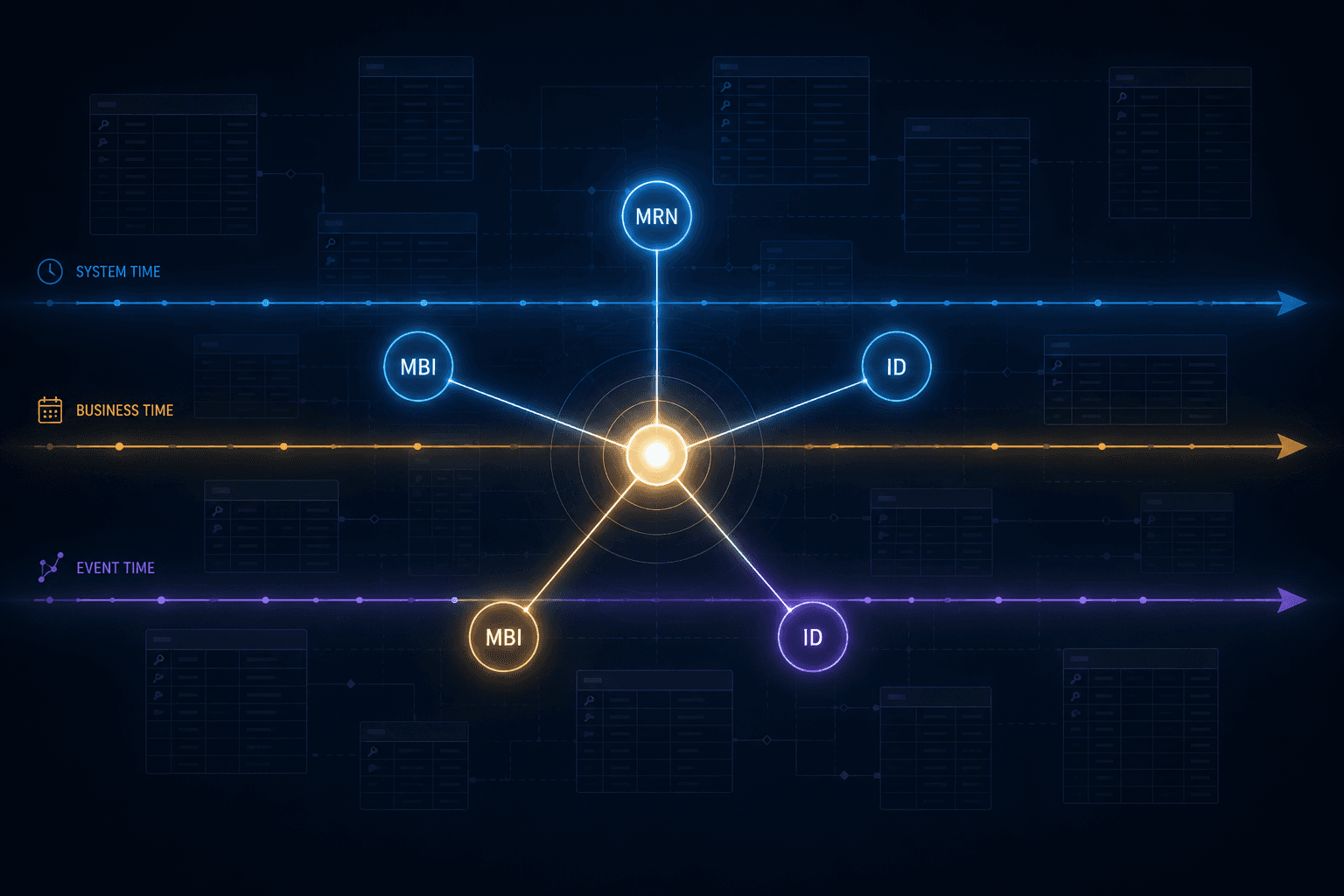
HL7v2 solved this decades ago. PID-3 — the patient identifier field in every HL7v2 message — is a repeating field. One patient, many identifiers, each qualified by an assigning authority and an identifier type code. A hospital issues an MRN. CMS issues an MBI. A payer issues a subscriber ID. They all point to the same person, and PID-3 stores them as parallel spokes off a single hub.
The 834 and 270 do the same thing implicitly — they just lack the metadata. So the table I built is the metadata HL7v2 always had:
CREATE TABLE person_identifiers (
    person_id           UUID REFERENCES persons(id),
    assigning_authority TEXT NOT NULL,   -- CMS, payer name, hospital OID
    id_type             TEXT NOT NULL,   -- MBI, subscriber_id, MRN, HICN
    identifier_value    TEXT NOT NULL,
    effective_start     DATE NOT NULL,
    effective_end       DATE,            -- NULL = still active
    source_transaction_id UUID REFERENCES raw_files(id),
    status              TEXT NOT NULL DEFAULT 'active'
);Every identifier traces back to the raw file that asserted it. Every identifier has a lifecycle — active, superseded, disputed. And person_id — the internal UUID that ties the spokes together — never leaves the platform. Downstream systems keep using their own identifiers. The spoke table is an internal resolution artifact, and keeping it internal is what lets us change our mind about a link without breaking every system that references us.
Two sisters. Same last name, same date of birth, same address, same subscriber contract — their parent's employer plan. The only difference in the enrollment file was first name and a two-character person code suffix. A composite key matcher — hash the SSN, match on DOB, fuzzy-match the name — produced a confident link. One record. Two girls' medical histories collapsed into one.
A false split is a duplicate record. Annoying, fixable, low-risk. A false merge is one person's pharmacy history attached to another person's clinical record. In Medicare, that's a CMS reportable event.
The spoke table prevents this by design. Resolution runs in tiers: deterministic first, probabilistic later, policy always. The deterministic tier — exact match on (assigning_authority, id_type, identifier_value) — resolves the large majority of volume at near-zero risk. MBI is the strongest anchor in a Medicare population: issued by CMS, unique per beneficiary, present across most inbound transactions. Subscriber ID plus person code handles the 834/270 dependent case cleanly, including twins, because person code is how the standard distinguishes dependents on the same contract.
Every link decision is stored as an event — method, score, actor, timestamp, and the field values as they stood at decision time. Merges are survivorship pointers, never physical record collapse. Unmerging a physically merged person record eighteen months later is the single most painful failure mode in this space. The spoke table means it never has to happen.
The Branch Test
Six tables, and the same design question on every column: typed or JSONB?
The instinct is to type what the implementation guide defines and put everything else in JSONB. That's the wrong cut. The right test is a single question: does code branch on this value?
If eligibility logic reads a field, if reconciliation compares it, if span calculation depends on it, if a downstream response references it — typed column with a constraint. If the field exists for pass-through, reporting, or because a payer asked us not to lose it — JSONB.
| Gets a typed column | Goes in payer_extensions (JSONB) |
|---|---|
| Maintenance type code (INS03) | Employer hire date |
| Maintenance reason code (INS04) | Department code |
| Benefit status | Salary band |
| Coverage date spans (DTP*348/349) | Location identifiers |
| Insurance line code (HD03) | Any Loop 2750 REF*ZZ pair |
| Subscriber/dependent relationship (INS02) | Companion guide extensions |
The JSONB half isn't a compromise. Loop 2750 in the 834 spec is literally a key-value bag by construction — N1*75 plus REF*ZZ reporting-category pairs. Employer hire dates, department codes, salary bands: they arrive as name-value pairs and JSONB stores them as name-value pairs. No impedance mismatch.
The typed half covers what drives behavior. Coverage date spans are real date columns because a string comparison in that path is a production defect waiting for a leap year. Maintenance type code is a constrained enum because INS03=024 means "cancellation or termination" and the maintenance reason code tells you which — if those values live in a JSONB bag, a typo silently changes someone's enrollment status.
Three disciplines keep JSONB honest. A schema registry per payer validates extensions at ingest — unvalidated JSONB accumulates typos, casing drift, and silently renamed keys. The original transaction is stored separately, immutably, so JSONB is a deliberate modeling choice rather than an insurance policy against data loss. And a promotion path: when a JSONB key starts being read by logic, it earns a typed column via migration. That promotion is someone's job, not something that happens by itself.
Three Clocks
Every enrollment platform stores effective dates. Coverage starts January 1st, terminates December 31st. Those are the dates the world cares about — when the coverage was true.
That's one clock. Healthcare data needs three.
Let me walk through a real scenario. A member named Priya enrolls in a Medicare Advantage plan. The January 834 arrives, the system processes it, and here's her coverage row:
| valid_from | valid_to | benefit_status | recorded_at |
|---|---|---|---|
| 2026-01-01 | NULL | active | Jan 15, 8:00 AM |
One clock. Valid time — when coverage is active in the world. This is what most enrollment systems store, and for the simple case it's enough.
Then things get complicated.
On February 28th, a disenrollment transaction posts to Priya's record — effective January 31st. The system processes it. On March 3rd, a provider submits a claim for services on February 15th. The system denies it: no active coverage on that date. Denial issued, claim returned.
On April 20th, CMS sends a Transaction Reply Report — a TRR, which is CMS's response to submitted transactions, communicating acceptances, rejections, and corrections back to plans. This one carries a correction: the disenrollment was in error. Priya's coverage is retroactively reinstated, effective January 1st with no end date.
Now the system needs to answer two questions simultaneously. Was the March 3rd denial correct? Yes — given what we knew, there was no coverage on February 15th. Should the claim be reprocessed? Also yes — because what we knew was wrong. Both facts have to coexist in the same table.
With only valid time — the single clock — the system can store the correction. But it destroys the original belief. There's no record that Priya was ever disenrolled, no way to explain why the claim was denied, and no audit trail for the grievance she's about to file.
That's why the canonical model stores three timestamps on every coverage row:
| Clock | Column | What it answers |
|---|---|---|
| Valid time | valid_from, valid_to | When was the coverage active in the world? |
| Transaction time | recorded_at | When did we come to believe it? |
| Source time | source_transaction_dt | When did the source system assert it? |
Here's what Priya's coverage looks like with all three clocks. Three rows for one person's coverage — each row is a belief the system held at a different point in time:
| valid_from | valid_to | recorded_at | source_dt | superseded_at | What this row means |
|---|---|---|---|---|---|
| 2026-01-01 | NULL | Jan 15 | Jan 14 | Feb 28 | Original enrollment — believed until Feb 28 |
| 2026-01-01 | 2026-01-31 | Feb 28 | Feb 27 | Apr 20 | Disenrollment — believed until Apr 20 |
| 2026-01-01 | NULL | Apr 20 | Apr 19 | NULL | Reinstatement — current belief |
Now the system can answer anything. "Was Priya covered on February 15th?" Query the current belief: yes. "Was she covered on February 15th as of March 3rd when the claim denied?" Query what we believed on March 3rd: no — the second row was the active belief, and it terminated January 31st. Both answers are correct, for different moments in time.
Valid time is the clock the domain forces on us anyway — every coverage span has effective and termination dates. Transaction time is what makes bitemporality work — it separates "what is true" from "when we learned it." Source time is the clock most systems forget: the source_dt column in Priya's rows shows the 834 and TRR were generated a day before we processed them. Late-arriving and out-of-order files are common enough that recorded_at and source_transaction_dt regularly diverge. Without source time, a file processed Thursday that was actually generated before one processed Tuesday silently wins by last-write, and nobody can detect the sequence was wrong.
The schema answers a question no single system can answer on its own: what did we believe, when did we believe it, and were we right?
Not everything needs all three clocks. The model tiers bitemporality by consequence:
- Fully bitemporal — anything a payment or claim decision depends on. Coverage spans, plan assignment, benefit status, premium, eligibility-driving demographics. These are the tables where CMS reconciliation, retro adjustments, and appeals land.
- Soft temporal — contact preferences, correspondence addresses, communication opt-ins.
updated_atis enough. Retroactive correctness carries no financial or regulatory consequence. - Neither — reference data and code sets. Versioned, not temporalized.
One convention that prevents more bugs than any validation rule: half-open intervals. Coverage runs [January 1, February 1) — the start date is inclusive, the end date is exclusive. No inclusive end dates, no 9999-12-31 sentinels, and NULL means open-ended. This sounds pedantic until you've spent a shift debugging a one-day coverage gap between two spans that both claim to include January 31st.
Postgres enforces this at the database level with daterange and a GiST exclusion constraint. Two coverage rows for the same person, plan, and coverage type cannot have overlapping valid ranges. The database rejects the insert before application code has a chance to be wrong.
The Schema That Contradicts Itself
Look at Priya's three rows again. The first and third both have valid_from = 2026-01-01 and valid_to = NULL. Their valid ranges overlap completely. That's the whole point of a correction — the new belief covers the same time period as the old one.
The exclusion constraint prevents exactly this. It exists to stop the database from storing two active coverage spans that claim a member was enrolled in the same plan for the same dates — which would double-count benefits, break premium billing, and produce wrong eligibility responses. That constraint is necessary.
But so is the correction. Both design decisions were right. They couldn't both be implemented as written.
The resolution is the superseded_at column — the fourth timestamp. When Priya's reinstatement arrives on April 20th, the system does two things in a single atomic transaction:
- Stamps
superseded_at = Apr 20on the old disenrollment row (row 2) - Inserts the new reinstatement row (row 3) with
superseded_at = NULL
The exclusion constraint becomes partial — it only prevents overlaps among rows we currently believe:
ALTER TABLE coverage
    ADD CONSTRAINT no_overlapping_current_coverage
    EXCLUDE USING gist (
        person_id WITH =,
        plan_id WITH =,
        coverage_type WITH =,
        daterange(valid_from, valid_to, '[)') WITH &&
    ) WHERE (superseded_at IS NULL);
The WHERE (superseded_at IS NULL) clause is doing all the work. Row 1 and row 2 have superseded_at set — they're historical beliefs, excluded from the constraint. Only row 3 is current. No overlap among current beliefs, constraint satisfied, correction stored, audit trail preserved.
Most application code never touches any of this. A coverage_current view returns only rows where superseded_at IS NULL — for Priya, that's one row showing active coverage from January 1st. A coverage_as_of() function takes a valid date and a knowledge date — "was Priya covered on Feb 15 as of March 3rd?" — and returns exactly the right answer. The bitemporal machinery stays in the database. The queries stay simple.
Where This Pays for Itself: Premium Billing
The schema design sounds academic until money is involved. Follow Priya's timeline through the billing system.
Priya pays $150 per month for her plan premium — a Medicare Advantage plan with Part D, dental, and vision benefits. When the enrollment processes in January, billing generates an invoice. January: $150, paid. Everything is clean.
On February 28th, the disenrollment arrives. Billing stops. February's premium is reversed — or never invoiced, depending on when in the cycle the transaction processed. March and April: no invoice generated.
On April 20th, the TRR reinstates Priya retroactively to January 1st. Now the plan needs to retro-bill three months of premiums. But here's the problem a single-clock system can't solve cleanly:
| Month | What happened | What billing needs to do |
|---|---|---|
| January | Invoiced $150, Priya paid | Nothing — already settled |
| February | Reversed or never invoiced after disenrollment | Re-invoice $150 |
| March | Never invoiced | Invoice $150 |
| April | Never invoiced | Invoice $150 |
| Retro-bill total | $450 |
A system with only valid time sees Priya as "active since January 1st" and might re-bill January too — a $600 invoice instead of $450. Priya disputes it. Someone investigates. Hours of reconciliation work because the system doesn't know that January was already billed under a previous belief.
With bitemporality, the billing calculation is a query: what did we believe between the old recorded_at and the new one? The disenrollment row tells billing that coverage was believed terminated from February 28th onward. The reinstatement row tells billing that belief changed on April 20th. The delta — February, March, April — is the retro-bill. January was never in question because it was billed under the original enrollment belief, which was never superseded during its billing period.
The same pattern handles retroactive disenrollments in the other direction. If Priya's coverage should have ended March 31st but the disenrollment doesn't process until May, the plan has already invoiced April and May premiums. Bitemporality tells the reconciliation engine exactly which months to credit back — the months where the old belief (active) and the new belief (terminated March 31st) disagree — without touching months where both beliefs agree.
This is why bitemporality isn't a theoretical exercise. Every retro adjustment, every TRR, every late-arriving 834 creates a billing delta. The schema either calculates it or someone calculates it by hand.
Classic invoice engines don't have this luxury. They run a recompute-and-compare cycle — re-price every member across every retro month (often 36 months deep), diff the result against the prior billing snapshot row by row, and generate credit/debit pairs for anything that changed. The engine does all that work because it doesn't know what changed — it has to rebuild the world to discover the delta. With bitemporality, the delta is the data. The superseded row and its replacement tell you exactly what changed, which fields differ, and which months need adjustment — one query against recorded_at and superseded_at instead of repricing millions of member-months to find the few hundred that moved.
Where This Pays for Itself: Hospital Eligibility
The premium scenario is the payer's problem. Here's the provider's.
Priya walks into Memorial Hospital's emergency department on March 10th — twelve days after her disenrollment was processed, six weeks before the TRR corrects it. The hospital knows her by her Medical Record Number: MH-2024-8891. That MRN means nothing to her insurance plan.
Before treating her, the hospital sends a 270 eligibility inquiry. This is where the spoke table earns its place. The payer's system doesn't store MRNs — it stores member IDs and subscriber IDs. But the spoke table has both: one row mapping MH-2024-8891 to Priya's person_id (sourced from a prior HL7v2 ADT message), another mapping her member ID to the same person_id (sourced from the 834). The resolution is a lookup, not a reconciliation project.
The coverage query runs against the current belief: terminated January 31st. The 271 comes back — not eligible. The hospital now has a decision. Treat Priya as self-pay and send her a $14,000 ER bill? Admit her and carry the financial risk? Ask her to call Medicare from the waiting room?
This happens every day, across thousands of hospitals.
The schema can't prevent the wrong answer on March 10th — the disenrollment is the current belief, and the 271 correctly reflects it. But when the TRR arrives on April 20th, the correction triggers a specific recovery path. The spoke table resolves MH-2024-8891 to Priya's person_id. Bitemporality identifies every claim that was denied during the window between the wrong disenrollment (February 28th) and the correction (April 20th) for coverage dates after January 31st. The reprocessing engine doesn't search — it queries: coverage_as_of('2026-03-10', '2026-03-03') returns "not covered" (what we believed when we denied), coverage_as_of('2026-03-10', NOW()) returns "covered" (what we know now). The delta between those two answers is the list of claims to reprocess.
Without the spoke table, the hospital's MRN and the payer's member ID are unconnected strings in different databases, reconciled by a human on the phone. Without bitemporality, there's no record that the eligibility answer was ever different — the claim sits in a denial queue until someone manually investigates, if they ever do.
The spoke table is functioning as a Master Person Index here — resolving identifiers across organizations. That's deliberate, but scoped. The platform resolves identity across every format it has ingested: 834s, 270/271s, HL7v2 ADT messages. It doesn't try to be an enterprise MPI across systems it doesn't touch. The boundary is the ingest layer — if the platform hasn't seen the transaction, it can't resolve the identifier. That's a feature, not a limitation. An unbounded MPI is an unbounded liability.
The Clock That Drifted
The schema was designed. The migration applied cleanly. Two hundred and eight tests passed, all green.
I ran the suite a second time. Seven tests failed.
Same code, same data, same machine. The only difference was wall-clock time. I measured: Python's clock ran 0.9 milliseconds ahead of the Docker Postgres clock. On the first run, every test's recorded_at happened to land safely after the database's NOW(). On the second run, a few landed in the database's future.
Here's what happened. A test inserts Priya's coverage with recorded_at stamped by Python at 08:00:00.000:
| valid_from | recorded_at (Python) | Database NOW() at insert |
|---|---|---|
| 2026-01-01 | 08:00:00.000 | 07:59:59.999 |
Then the test calls coverage_as_of('2026-02-15', NOW()) — "what coverage exists as of right now?" The database evaluates NOW() as 07:59:59.999. The query filters for recorded_at <= NOW(). But 08:00:00.000 is after 07:59:59.999 — so the row the test just wrote is invisible. The database thinks it hasn't learned about it yet. The test fails: no coverage found.
Move the clocks forward a few milliseconds and the skew leans the other way — Python stamps 08:00:00.001, the database's NOW() returns 08:00:00.002, and everything passes. Same code, different millisecond.
The fix was straightforward: stop mixing clocks. Every stored timestamp now uses COALESCE($n, NOW()) — the Pydantic model defaults to None, and the database stamps its own time on insert. After the fix, Priya's row looks like this:
| valid_from | recorded_at (Database) | Database NOW() at query |
|---|---|---|
| 2026-01-01 | 07:59:59.999 | 07:59:59.999 |
One clock. No skew. The row is always visible to the query that follows the insert.
What the fix exposed was harder than the fix itself.
The original tests for the COALESCE pattern had a problem: most of them couldn't actually catch the regression they were written for. Consider a test for resolve_person, which looks up a person by identifier. The original code used date.today() in Python to check if an identifier was active. A test that inserts an identifier effective today and resolves it will pass — because date.today() in Python and CURRENT_DATE in Postgres are the same date for all but a few seconds around midnight, and only when the app server and database are in different timezones. The test documents the rule ("use the database clock") but can only catch a violation in a window measured in seconds per day.
So I wrote a different kind of test. One that parses the source file and asserts it contains no Python clock call at all — no datetime.now(), no date.today(), no default_factory that stamps a timestamp. Deterministic. And it fails on exactly the regression that would reintroduce the bug: add default_factory=_now back to any model's timestamp field, and the test names the line.
That exercise clarified something I hadn't thought about carefully enough — three kinds of temporal tests, and only one of them is a real guard:
| Kind | What it does | Can it miss the bug? |
|---|---|---|
| Static guard | Parses source code, asserts a structural rule | No — catches the regression regardless of clock state |
| Contract test | Verifies behavior independent of clock direction | No — passes regardless of which clock is faster |
| Symptom test | Only catches the bug when the clock skews the wrong way | Yes — passes in CI, passes locally, fails on a different host at 11:59 PM |
The symptom tests look like protection. They pass reliably, they pass in CI, they pass on first run. They fail intermittently, on a different host, or when the container's load is different. A test that documents a rule without catching the violation is the worst kind of false confidence — it makes you think you're covered when the guard is a coincidence.
What the Schema Holds
Six tables. Three temporal clocks. A spoke model for identity. An exclusion constraint that contradicts bitemporality until a fourth timestamp resolves the contradiction. A schema registry stub for payer-specific JSONB. And a test suite that includes guards against its own assumptions — tests that catch regressions structurally, not by hoping the clock drifts the right direction.
The canonical model is Person, not Member. Coverage, not Enrollment. Identity resolution is a graph of qualified identifiers, not a composite key collision. Time has three meanings that the schema makes explicit in every row.
Provider, Encounter, Claim, and Payment exist as stubs — a primary key and a foreign key back to persons. They earn real columns when their parsers land. Designing a claims table before building a claims parser is how you end up redesigning the claims table after building the claims parser. The canonical model grows with the pipeline, not ahead of it.
In Part 4, I build the first parser — the X12 834 enrollment file that started this entire series. The file that arrives with three hundred member records, forty-seven of which failed because a companion guide variation didn't match the mapping table. The canonical model is ready to hold what the parser produces. The question now is whether the parser can produce it.